How Ensemle Learning Works Well Then Normal

Introduction

When yous want to purchase a new machine, will you walk upward to the outset car shop and purchase one based on the communication of the dealer? It'due south highly unlikely.

You lot would likely browser a few web portals where people have posted their reviews and compare dissimilar car models, checking for their features and prices. You will also probably ask your friends and colleagues for their opinion. In short, you lot wouldn't directly reach a conclusion, but will instead make a conclusion considering the opinions of other people also.

Ensemble models in motorcar learning operate on a similar thought. They combine the decisions from multiple models to meliorate the overall performance. This can be accomplished in various ways, which yous volition detect in this article.

The objective of this commodity is to introduce the concept of ensemble learning and understand the algorithms which use this technique. To cement your agreement of this various topic, we volition explain the advanced algorithms in Python using a hands-on case study on a real-life trouble.

Note: This article assumes a basic understanding of Machine Learning algorithms. I would recommend going through this article to familiarize yourself with these concepts. Yous tin also learn almost ensemble learning chapter-wise past enrolling in this free course:

Ensemble Learning and Ensemble Learning Techniques

Are yous a beginner looking for a place to start your journey in data science and machine learning? Presenting two comprehensive courses, full of cognition and data scientific discipline learning, curated just for you!

Practical Machine Learning Course
Certified AI & ML Blackbelt+ Plan

Introduction to Ensemble Learning
Basic Ensemble Techniques
2.i Max Voting
2.ii Averaging
2.3 Weighted Average
Advanced Ensemble Techniques
3.ane Stacking
3.2 Blending
three.three Bagging
3.4 Boosting
Algorithms based on Bagging and Boosting
4.i Bagging meta-reckoner
4.2 Random Woods
4.iii AdaBoost
4.four GBM
four.5 XGB
4.6 Calorie-free GBM
iv.7 CatBoost

1. Introduction to Ensemble Learning

Let's understand the concept of ensemble learning with an example. Suppose you are a movie director and you take created a short movie on a very important and interesting topic. Now, y'all desire to have preliminary feedback (ratings) on the movie before making it public. What are the possible ways past which you lot tin do that?

A: You may enquire ane of your friends to rate the movie for yous.
Now information technology'south entirely possible that the person you take chosen loves you very much and doesn't want to break your heart by providing a 1-star rating to the horrible piece of work yous have created.

B: Another way could be past asking five colleagues of yours to rate the pic.
This should provide a ameliorate idea of the movie. This method may provide honest ratings for your movie. But a problem still exists. These five people may not be "Bailiwick Thing Experts" on the topic of your motion picture. Sure, they might empathise the cinematography, the shots, or the sound, but at the same time may not exist the all-time judges of dark humour.

C: How about asking fifty people to rate the film?
Some of which can be your friends, some of them can be your colleagues and some may even be total strangers.

The responses, in this case, would be more generalized and diversified since now y'all have people with different sets of skills. And every bit it turns out – this is a amend approach to get honest ratings than the previous cases nosotros saw.

With these examples, you tin can infer that a various group of people are likely to make better decisions as compared to individuals. Similar is true for a diverse set of models in comparing to single models. This diversification in Machine Learning is accomplished past a technique called Ensemble Learning.

Now that you take got a gist of what ensemble learning is – let us look at the diverse techniques in ensemble learning along with their implementations.

two. Simple Ensemble Techniques

In this department, nosotros will look at a few simple only powerful techniques, namely:

Max Voting
Averaging
Weighted Averaging

2.1 Max Voting

The max voting method is generally used for classification problems. In this technique, multiple models are used to make predictions for each data point. The predictions by each model are considered as a 'vote'. The predictions which we get from the majority of the models are used as the final prediction.

For example, when you asked 5 of your colleagues to rate your movie (out of 5); we'll assume three of them rated it as 4 while two of them gave it a 5. Since the majority gave a rating of 4, the concluding rating will be taken every bit 4. You lot can consider this as taking the mode of all the predictions.

The result of max voting would be something similar this:

Colleague 1	Colleague 2	Colleague 3	Colleague 4	Colleague 5	Last rating
5	4	v	iv	four	4

Sample Lawmaking:

Here x_train consists of independent variables in preparation data, y_train is the target variable for training data. The validation set is x_test (independent variables) and y_test (target variable) .

          model1 = tree.DecisionTreeClassifier() model2 = KNeighborsClassifier() model3= LogisticRegression()          model1.fit(x_train,y_train) model2.fit(x_train,y_train) model3.fit(x_train,y_train)  pred1=model1.predict(x_test) pred2=model2.predict(x_test) pred3=model3.predict(x_test)  final_pred = np.assortment([]) for i in range(0,len(x_test)):     final_pred = np.suspend(final_pred, mode([pred1[i], pred2[i], pred3[i]]))

Alternatively, you can use "VotingClassifier" module in sklearn as follows:

from sklearn.ensemble import VotingClassifier model1 = LogisticRegression(random_state=i) model2 = tree.DecisionTreeClassifier(random_state=i) model = VotingClassifier(estimators=[('lr', model1), ('dt', model2)], voting='hard') model.fit(x_train,y_train) model.score(x_test,y_test)

2.ii Averaging

Similar to the max voting technique, multiple predictions are made for each data bespeak in averaging. In this method, we accept an average of predictions from all the models and apply it to make the last prediction. Averaging can exist used for making predictions in regression issues or while computing probabilities for classification bug.

For instance, in the below case, the averaging method would take the average of all the values.

i.east. (5+four+5+iv+iv)/5 = 4.4

Colleague 1	Colleague 2	Colleague 3	Colleague four	Colleague 5	Concluding rating
5	4	v	four	iv	four.4

Sample Lawmaking:

model1 = tree.DecisionTreeClassifier() model2 = KNeighborsClassifier() model3= LogisticRegression()  model1.fit(x_train,y_train) model2.fit(x_train,y_train) model3.fit(x_train,y_train)  pred1=model1.predict_proba(x_test) pred2=model2.predict_proba(x_test) pred3=model3.predict_proba(x_test)  finalpred=(pred1+pred2+pred3)/3

2.three Weighted Average

This is an extension of the averaging method. All models are assigned different weights defining the importance of each model for prediction. For example, if two of your colleagues are critics, while others have no prior experience in this field, then the answers by these two friends are given more importance equally compared to the other people.

The result is calculated every bit [(5*0.23) + (four*0.23) + (5*0.xviii) + (4*0.xviii) + (4*0.eighteen)] = four.41.

	Colleague i	Colleague 2	Colleague 3	Colleague 4	Colleague v	Last rating
weight	0.23	0.23	0.18	0.xviii	0.18
rating	v	four	5	4	4	iv.41

Sample Lawmaking:

model1 = tree.DecisionTreeClassifier() model2 = KNeighborsClassifier() model3= LogisticRegression()  model1.fit(x_train,y_train) model2.fit(x_train,y_train) model3.fit(x_train,y_train)  pred1=model1.predict_proba(x_test) pred2=model2.predict_proba(x_test) pred3=model3.predict_proba(x_test)  finalpred=(pred1*0.3+pred2*0.iii+pred3*0.iv)

3. Advanced Ensemble techniques

Now that we have covered the basic ensemble techniques, permit's move on to agreement the advanced techniques.

3.ane Stacking

Stacking is an ensemble learning technique that uses predictions from multiple models (for instance decision tree, knn or svm) to build a new model. This model is used for making predictions on the test gear up. Beneath is a footstep-wise explanation for a simple stacked ensemble:

The train set is separate into x parts.
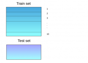
A base of operations model (suppose a determination tree) is fitted on nine parts and predictions are made for the 10th part. This is done for each part of the train set.
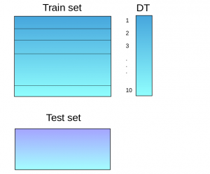
The base model (in this example, decision tree) is then fitted on the whole train dataset.
Using this model, predictions are made on the test ready.
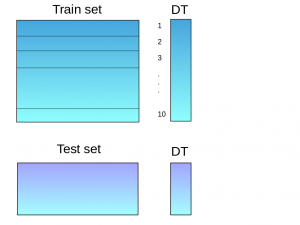
Steps two to 4 are repeated for some other base model (say knn) resulting in some other set of predictions for the train set up and test set.
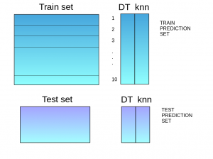
The predictions from the railroad train prepare are used equally features to build a new model.
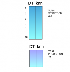
This model is used to brand final predictions on the examination prediction set up.

Sample lawmaking:

Nosotros first ascertain a function to make predictions on n-folds of railroad train and test dataset. This office returns the predictions for train and test for each model.

def Stacking(model,train,y,test,n_fold):    folds=StratifiedKFold(n_splits=n_fold,random_state=1)    test_pred=np.empty((test.shape[0],ane),float)    train_pred=np.empty((0,1),float)    for train_indices,val_indices in folds.split(train,y.values):       x_train,x_val=railroad train.iloc[train_indices],train.iloc[val_indices]       y_train,y_val=y.iloc[train_indices],y.iloc[val_indices]        model.fit(X=x_train,y=y_train)       train_pred=np.append(train_pred,model.predict(x_val))       test_pred=np.suspend(test_pred,model.predict(exam))     return test_pred.reshape(-1,one),train_pred

Now we'll create two base models – conclusion tree and knn.

model1 = tree.DecisionTreeClassifier(random_state=1)  test_pred1 ,train_pred1=Stacking(model=model1,n_fold=ten, train=x_train,exam=x_test,y=y_train)  train_pred1=pd.DataFrame(train_pred1) test_pred1=pd.DataFrame(test_pred1)

model2 = KNeighborsClassifier()  test_pred2 ,train_pred2=Stacking(model=model2,n_fold=10,train=x_train,test=x_test,y=y_train)  train_pred2=pd.DataFrame(train_pred2) test_pred2=pd.DataFrame(test_pred2)

Create a third model, logistic regression, on the predictions of the decision tree and knn models.

df = pd.concat([train_pred1, train_pred2], axis=1) df_test = pd.concat([test_pred1, test_pred2], axis=1)  model = LogisticRegression(random_state=ane) model.fit(df,y_train) model.score(df_test, y_test)

In order to simplify the above explanation, the stacking model nosotros take created has just ii levels. The determination tree and knn models are built at level zero, while a logistic regression model is built at level 1. Feel free to create multiple levels in a stacking model.

3.ii Blending

Blending follows the same approach as stacking but uses simply a holdout (validation) set from the railroad train set to brand predictions. In other words, different stacking, the predictions are fabricated on the holdout set just. The holdout gear up and the predictions are used to build a model which is run on the test fix. Here is a detailed explanation of the blending process:

The train ready is split into training and validation sets.
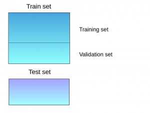
Model(due south) are fitted on the training prepare.
The predictions are made on the validation set and the test set up.
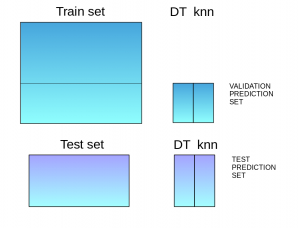
The validation set and its predictions are used as features to build a new model.
This model is used to make last predictions on the exam and meta-features.

Sample Code:

We'll build 2 models, determination tree and knn, on the train set in gild to make predictions on the validation set.

model1 = tree.DecisionTreeClassifier() model1.fit(x_train, y_train) val_pred1=model1.predict(x_val) test_pred1=model1.predict(x_test) val_pred1=pd.DataFrame(val_pred1) test_pred1=pd.DataFrame(test_pred1)  model2 = KNeighborsClassifier() model2.fit(x_train,y_train) val_pred2=model2.predict(x_val) test_pred2=model2.predict(x_test) val_pred2=pd.DataFrame(val_pred2) test_pred2=pd.DataFrame(test_pred2)

Combining the meta-features and the validation set, a logistic regression model is congenital to make predictions on the exam set.

df_val=pd.concat([x_val, val_pred1,val_pred2],axis=1) df_test=pd.concat([x_test, test_pred1,test_pred2],axis=1)  model = LogisticRegression() model.fit(df_val,y_val) model.score(df_test,y_test)

3.3 Bagging

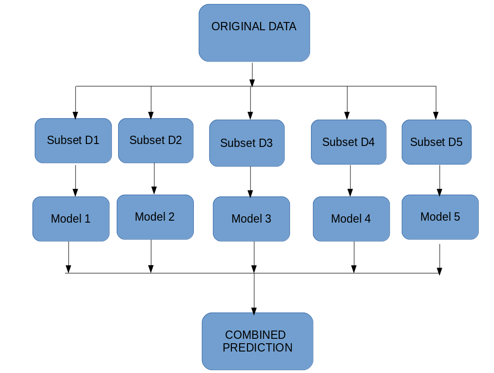
The idea behind bagging is combining the results of multiple models (for case, all determination trees) to get a generalized outcome. Hither's a question: If you create all the models on the same set of data and combine it, will it be useful? There is a high chance that these models will give the aforementioned result since they are getting the same input. And so how can we solve this trouble? One of the techniques is bootstrapping.

Bootstrapping is a sampling technique in which we create subsets of observations from the original dataset, with replacement. The size of the subsets is the same as the size of the original set.

Bagging (or Bootstrap Aggregating) technique uses these subsets (bags) to get a off-white idea of the distribution (consummate ready). The size of subsets created for bagging may be less than the original ready.

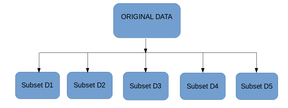
Multiple subsets are created from the original dataset, selecting observations with replacement.
A base of operations model (weak model) is created on each of these subsets.
The models run in parallel and are independent of each other.
The concluding predictions are determined by combining the predictions from all the models.

3.4 Boosting

Before nosotros go farther, here's some other question for y'all: If a data point is incorrectly predicted past the commencement model, and so the side by side (probably all models), will combining the predictions provide ameliorate results? Such situations are taken intendance of by boosting.

Boosting is a sequential process, where each subsequent model attempts to correct the errors of the previous model. The succeeding models are dependent on the previous model. Allow's understand the way boosting works in the below steps.

A subset is created from the original dataset.
Initially, all data points are given equal weights.
A base model is created on this subset.
This model is used to make predictions on the whole dataset.
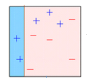
Errors are calculated using the bodily values and predicted values.
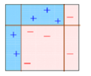
The observations which are incorrectly predicted, are given higher weights.
(Hither, the iii misclassified bluish-plus points will be given higher weights)
Another model is created and predictions are made on the dataset.
(This model tries to correct the errors from the previous model)
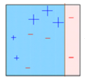
Similarly, multiple models are created, each correcting the errors of the previous model.
The final model (strong learner) is the weighted hateful of all the models (weak learners). Thus, the boosting algorithm combines a number of weak learners to form a strong learner. The individual models would not perform well on the entire dataset, but they work well for some part of the dataset. Thus, each model actually boosts the functioning of the ensemble.

4. Algorithms based on Bagging and Boosting

Bagging and Boosting are ii of the most commonly used techniques in car learning. In this section, we volition look at them in detail. Post-obit are the algorithms we will be focusing on:

Bagging algorithms:

Bagging meta-estimator
Random forest

Boosting algorithms:

AdaBoost
GBM
XGBM
Light GBM
CatBoost

For all the algorithms discussed in this section, we volition follow this procedure:

Introduction to the algorithm
Sample lawmaking
Parameters

For this article, I have used the Loan Prediction Problem. You can download the dataset from here . Please note that a few lawmaking lines (reading the data, splitting into train-test sets, etc.) volition be the same for each algorithm. In social club to avoid repetition, I accept written the code for the same below, and further discussed merely the code for the algorithm.

#importing of import packages import pandas every bit pd import numpy every bit np  #reading the dataset df=pd.read_csv("/dwelling/user/Desktop/train.csv")  #filling missing values df['Gender'].fillna('Male', inplace=True)

Similarly, fill up values for all the columns. EDA, missing values and outlier treatment has been skipped for the purposes of this commodity. To understand these topics, you tin can get through this commodity: Ultimate guide for Data Exploration in Python using NumPy, Matplotlib and Pandas .

#split dataset into train and test  from sklearn.model_selection import train_test_split train, test = train_test_split(df, test_size=0.iii, random_state=0)  x_train=railroad train.drib('Loan_Status',axis=1) y_train=train['Loan_Status']  x_test=test.drib('Loan_Status',axis=one) y_test=examination['Loan_Status']  #create dummies x_train=pd.get_dummies(x_train) x_test=pd.get_dummies(x_test)

Let's jump into the bagging and boosting algorithms!

iv.ane Bagging meta-computer

Bagging meta-calculator is an ensembling algorithm that can be used for both classification (BaggingClassifier) and regression (BaggingRegressor) bug. It follows the typical bagging technique to make predictions. Following are the steps for the bagging meta-estimator algorithm:

Random subsets are created from the original dataset (Bootstrapping).
The subset of the dataset includes all features.
A user-specified base estimator is fitted on each of these smaller sets.
Predictions from each model are combined to go the final issue.

Code:

from sklearn.ensemble import BaggingClassifier from sklearn import tree model = BaggingClassifier(tree.DecisionTreeClassifier(random_state=1)) model.fit(x_train, y_train) model.score(x_test,y_test) 0.75135135135135134

Sample lawmaking for regression problem:

from sklearn.ensemble import BaggingRegressor model = BaggingRegressor(tree.DecisionTreeRegressor(random_state=1)) model.fit(x_train, y_train) model.score(x_test,y_test)

Parameters used in the algorithms:

base_estimator:
- It defines the base figurer to fit on random subsets of the dataset.
- When zippo is specified, the base of operations estimator is a determination tree.
n_estimators:
- Information technology is the number of base estimators to be created.
- The number of estimators should be advisedly tuned as a large number would have a very long time to run, while a very small number might non provide the best results.
max_samples:
- This parameter controls the size of the subsets.
- It is the maximum number of samples to train each base calculator.
max_features:
- Controls the number of features to draw from the whole dataset.
- Information technology defines the maximum number of features required to railroad train each base estimator.
n_jobs:
- The number of jobs to run in parallel.
- Prepare this value equal to the cores in your system.
- If -1, the number of jobs is set to the number of cores.

random_state:
- Information technology specifies the method of random split. When random state value is same for 2 models, the random selection is aforementioned for both models.
- This parameter is useful when you lot want to compare dissimilar models.

4.2 Random Forest

Random Woods is some other ensemble machine learning algorithm that follows the bagging technique. It is an extension of the bagging estimator algorithm. The base estimators in random woods are decision trees. Different bagging meta figurer, random forest randomly selects a set of features which are used to decide the best split at each node of the conclusion tree.

Looking at it step-past-pace, this is what a random forest model does:

Random subsets are created from the original dataset (bootstrapping).
At each node in the decision tree, only a random set of features are considered to decide the best dissever.
A decision tree model is fitted on each of the subsets.
The terminal prediction is calculated past averaging the predictions from all decision trees.

Notation: The conclusion trees in random forest tin can be congenital on a subset of data and features. Particularly, the sklearn model of random forest uses all features for decision tree and a subset of features are randomly selected for splitting at each node.

To sum up, Random forest r andomly selects data points and features, and builds multiple copse (Forest) .

Code:

Parameters

n_estimators:
- It defines the number of conclusion trees to be created in a random forest.
- Generally, a higher number makes the predictions stronger and more than stable, just a very large number can event in college training time.
benchmark:
- It defines the function that is to be used for splitting.
- The office measures the quality of a divide for each characteristic and chooses the best split.
max_features :
- Information technology defines the maximum number of features immune for the carve up in each determination tree.
- Increasing max features normally improve performance simply a very high number can decrease the diversity of each tree.
max_depth:
- Random wood has multiple decision copse. This parameter defines the maximum depth of the trees.
min_samples_split:
- Used to define the minimum number of samples required in a leaf node before a split is attempted.
- If the number of samples is less than the required number, the node is not carve up.
min_samples_leaf:
- This defines the minimum number of samples required to be at a foliage node.
- Smaller leaf size makes the model more than prone to capturing racket in train information.
max_leaf_nodes:
- This parameter specifies the maximum number of leaf nodes for each tree.
- The tree stops splitting when the number of leaf nodes becomes equal to the max leaf node.
n_jobs:
- This indicates the number of jobs to run in parallel.
- Set value to -ane if yous want it to run on all cores in the system.
random_state:
- This parameter is used to define the random selection.
- It is used for comparing between various models.

4.3 AdaBoost

Adaptive boosting or AdaBoost is one of the simplest boosting algorithms. Usually, conclusion trees are used for modelling. Multiple sequential models are created, each correcting the errors from the last model. AdaBoost assigns weights to the observations which are incorrectly predicted and the subsequent model works to predict these values correctly.

Below are the steps for performing the AdaBoost algorithm:

Initially, all observations in the dataset are given equal weights.
A model is built on a subset of data.
Using this model, predictions are made on the whole dataset.
Errors are calculated past comparison the predictions and bodily values.
While creating the next model, higher weights are given to the data points which were predicted incorrectly.
Weights can be determined using the error value. For instance, higher the error more is the weight assigned to the observation.
This process is repeated until the fault function does non change, or the maximum limit of the number of estimators is reached.

Code:

from sklearn.ensemble import AdaBoostClassifier model = AdaBoostClassifier(random_state=ane) model.fit(x_train, y_train) model.score(x_test,y_test) 0.81081081081081086

Sample code for regression problem:

from sklearn.ensemble import AdaBoostRegressor model = AdaBoostRegressor() model.fit(x_train, y_train) model.score(x_test,y_test)

Parameters

base_estimators:
- It helps to specify the type of base of operations estimator, that is, the machine learning algorithm to exist used equally base learner.
n_estimators:
- It defines the number of base of operations estimators.
- The default value is 10, but you should keep a higher value to get better functioning.
learning_rate:
- This parameter controls the contribution of the estimators in the final combination.
- There is a trade-off between learning_rate and n_estimators.
max_depth:
- Defines the maximum depth of the individual reckoner.
- Tune this parameter for best performance.
n_jobs
- Specifies the number of processors it is allowed to use.
- Ready value to -one for maximum processors allowed.
random_state :
- An integer value to specify the random data split.
- A definite value of random_state will e'er produce aforementioned results if given with aforementioned parameters and training information.

four.4 Gradient Boosting (GBM)

Gradient Boosting or GBM is another ensemble auto learning algorithm that works for both regression and nomenclature problems. GBM uses the boosting technique, combining a number of weak learners to form a strong learner. Regression trees used every bit a base learner, each subsequent tree in series is built on the errors calculated by the previous tree.

We will use a simple case to understand the GBM algorithm. We have to predict the age of a group of people using the below data:

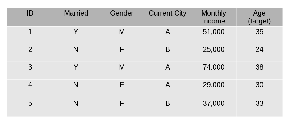
The mean age is assumed to be the predicted value for all observations in the dataset.
The errors are calculated using this hateful prediction and bodily values of age.
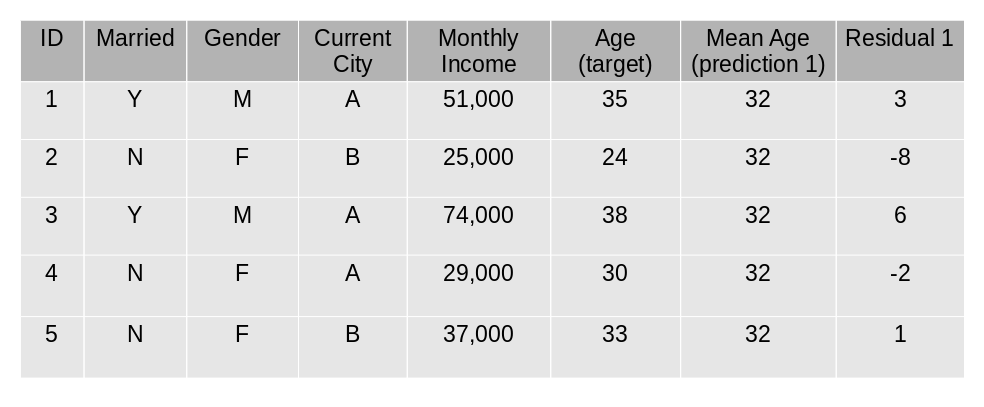
A tree model is created using the errors calculated above as target variable. Our objective is to find the best dissever to minimize the fault.
The predictions by this model are combined with the predictions 1.
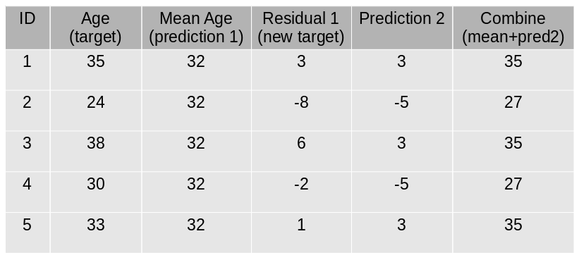
This value calculated in a higher place is the new prediction.
New errors are calculated using this predicted value and actual value.
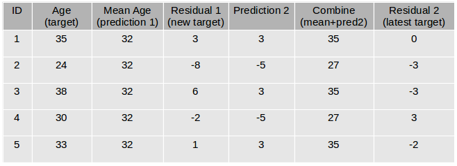
Steps 2 to 6 are repeated till the maximum number of iterations is reached (or fault function does non modify).

Lawmaking:

from sklearn.ensemble import GradientBoostingClassifier model= GradientBoostingClassifier(learning_rate=0.01,random_state=1) model.fit(x_train, y_train) model.score(x_test,y_test) 0.81621621621621621

Sample lawmaking for regression trouble:

from sklearn.ensemble import GradientBoostingRegressor model= GradientBoostingRegressor() model.fit(x_train, y_train) model.score(x_test,y_test)

Parameters

min_samples_split
- Defines the minimum number of samples (or observations) which are required in a node to be considered for splitting.
- Used to control over-fitting. Higher values forbid a model from learning relations which might exist highly specific to the particular sample selected for a tree.
min_samples_leaf
- Defines the minimum samples required in a last or leaf node.
- Generally, lower values should be chosen for imbalanced grade problems because the regions in which the minority class will be in the majority will exist very small.

min_weight_fraction_leaf
- Like to min_samples_leaf but defined as a fraction of the full number of observations instead of an integer.
max_depth
- The maximum depth of a tree.
- Used to control over-plumbing equipment equally higher depth will let the model to learn relations very specific to a item sample.
- Should exist tuned using CV.
max_leaf_nodes
- The maximum number of terminal nodes or leaves in a tree.
- Tin exist defined in place of max_depth. Since binary copse are created, a depth of 'northward' would produce a maximum of 2^n leaves.
- If this is defined, GBM will ignore max_depth.
max_features
- The number of features to consider while searching for the all-time split. These will be randomly selected.
- As a pollex-rule, the square root of the total number of features works great but we should check up to 30-40% of the full number of features.
- Higher values can lead to over-plumbing equipment but it generally depends on a case to case scenario.

4.v XGBoost

XGBoost (farthermost Slope Boosting) is an advanced implementation of the gradient boosting algorithm. XGBoost has proved to be a highly constructive ML algorithm, extensively used in motorcar learning competitions and hackathons. XGBoost has high predictive power and is virtually 10 times faster than the other slope boosting techniques. It also includes a diversity of regularization which reduces overfitting and improves overall functioning. Hence information technology is too known as 'regularized boosting' technique.

Permit us see how XGBoost is comparatively better than other techniques:

Regularization:
- Standard GBM implementation has no regularisation like XGBoost.
- Thus XGBoost also helps to reduce overfitting.
Parallel Processing:
- XGBoost implements parallel processing and is faster than GBM .
- XGBoost also supports implementation on Hadoop.
High Flexibility:
- XGBoost allows users to define custom optimization objectives and evaluation criteria adding a whole new dimension to the model.
Handling Missing Values:
- XGBoost has an in-built routine to handle missing values.
Tree Pruning:
- XGBoost makes splits upwards to the max_depth specified and then starts pruning the tree backwards and removes splits beyond which there is no positive gain.
Built-in Cantankerous-Validation:
- XGBoost allows a user to run a cross-validation at each iteration of the boosting procedure and thus it is easy to get the exact optimum number of boosting iterations in a unmarried run.

Code:

Since XGBoost takes intendance of the missing values itself, you practice not take to impute the missing values. You can skip the step for missing value imputation from the code mentioned to a higher place. Follow the remaining steps as e'er and then utilise xgboost as below.

import xgboost as xgb model=xgb.XGBClassifier(random_state=1,learning_rate=0.01) model.fit(x_train, y_train) model.score(x_test,y_test) 0.82702702702702702

Sample lawmaking for regression problem:

import xgboost as xgb model=xgb.XGBRegressor() model.fit(x_train, y_train) model.score(x_test,y_test)

Parameters

nthread
- This is used for parallel processing and the number of cores in the system should be entered..
- If you lot wish to run on all cores, do not input this value. The algorithm will find information technology automatically.
eta
- Analogous to learning rate in GBM.
- Makes the model more robust by shrinking the weights on each step.
min_child_weight
- Defines the minimum sum of weights of all observations required in a child.
- Used to control over-fitting. College values preclude a model from learning relations which might be highly specific to the detail sample selected for a tree.
max_depth
- It is used to define the maximum depth.
- College depth will allow the model to learn relations very specific to a particular sample.
max_leaf_nodes
- The maximum number of concluding nodes or leaves in a tree.
- Can be divers in identify of max_depth. Since binary copse are created, a depth of 'n' would produce a maximum of 2^n leaves.
- If this is defined, GBM will ignore max_depth.
gamma
- A node is split up simply when the resulting split gives a positive reduction in the loss function. Gamma specifies the minimum loss reduction required to brand a dissever.
- Makes the algorithm conservative. The values can vary depending on the loss function and should be tuned.
subsample
- Aforementioned as the subsample of GBM. Denotes the fraction of observations to be randomly sampled for each tree.
- Lower values brand the algorithm more conservative and foreclose overfitting but values that are too modest might pb to under-plumbing equipment.
colsample_bytree
- It is like to max_features in GBM.
- Denotes the fraction of columns to be randomly sampled for each tree.

iv.6 Light GBM

Before discussing how Calorie-free GBM works, let's first understand why we demand this algorithm when we have so many others (like the ones we accept seen above). Calorie-free GBM beats all the other algorithms when the dataset is extremely big. Compared to the other algorithms, Calorie-free GBM takes lesser time to run on a huge dataset.

LightGBM is a gradient boosting framework that uses tree-based algorithms and follows leaf-wise approach while other algorithms piece of work in a level-wise approach design. The images beneath will aid you understand the difference in a ameliorate way.

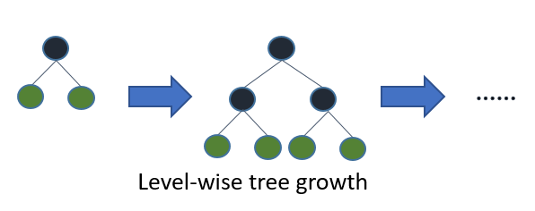
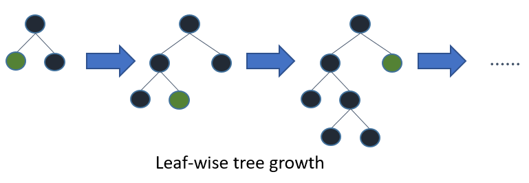
Leaf-wise growth may crusade over-fitting on smaller datasets but that can exist avoided past using the 'max_depth' parameter for learning. You can read more than about Lite GBM and its comparing with XGB in this commodity.

Code:

import lightgbm as lgb train_data=lgb.Dataset(x_train,label=y_train) #define parameters params = {'learning_rate':0.001} model= lgb.train(params, train_data, 100)  y_pred=model.predict(x_test) for i in range(0,185):    if y_pred[i]>=0.v:     y_pred[i]=1 else:     y_pred[i]=0 0.81621621621621621

Sample lawmaking for regression problem:

import lightgbm as lgb train_data=lgb.Dataset(x_train,label=y_train) params = {'learning_rate':0.001} model= lgb.train(params, train_data, 100) from sklearn.metrics import mean_squared_error rmse=mean_squared_error(y_pred,y_test)**0.5

Parameters

num_iterations:
- It defines the number of boosting iterations to exist performed.
num_leaves :
- This parameter is used to set the number of leaves to be formed in a tree.
- In example of Light GBM, since splitting takes place foliage-wise rather than depth-wise, num_leaves must exist smaller than 2^(max_depth), otherwise, it may lead to overfitting.
min_data_in_leaf :
- A very small value may crusade overfitting.
- It is besides one of the most important parameters in dealing with overfitting.
max_depth:
- It specifies the maximum depth or level up to which a tree can grow.
- A very loftier value for this parameter tin cause overfitting.
bagging_fraction:
- It is used to specify the fraction of data to be used for each iteration.
- This parameter is generally used to speed up the training.
max_bin :
- Defines the max number of bins that characteristic values will be bucketed in.
- A smaller value of max_bin tin save a lot of time equally information technology buckets the feature values in detached bins which is computationally inexpensive.

4.seven CatBoost

Treatment categorical variables is a tiresome process, specially when you lot have a big number of such variables. When your categorical variables have as well many labels (i.e. they are highly central), performing one-hot-encoding on them exponentially increases the dimensionality and it becomes really difficult to work with the dataset.

CatBoost tin can automatically deal with categorical variables and does non crave extensive data preprocessing like other machine learning algorithms. Here is an article that explains CatBoost in detail.

Code:

CatBoost algorithm effectively deals with categorical variables. Thus, yous should not perform one-hot encoding for chiselled variables. Merely load the files, impute missing values, and you're good to go.

from catboost import CatBoostClassifier model=CatBoostClassifier() categorical_features_indices = np.where(df.dtypes != np.float)[0] model.fit(x_train,y_train,cat_features=([ 0,  1, 2, three, 4, 10]),eval_set=(x_test, y_test)) model.score(x_test,y_test) 0.80540540540540539

Sample code for regression problem:

from catboost import CatBoostRegressor model=CatBoostRegressor() categorical_features_indices = np.where(df.dtypes != np.float)[0] model.fit(x_train,y_train,cat_features=([ 0,  1, 2, iii, four, x]),eval_set=(x_test, y_test)) model.score(x_test,y_test)

Parameters

loss_function:
- Defines the metric to be used for training.

iterations:
- The maximum number of trees that can be built.
- The terminal number of trees may exist less than or equal to this number.
learning_rate:
- Defines the learning rate.
- Used for reducing the gradient pace.
border_count:
- Information technology specifies the number of splits for numerical features.
- It is similar to the max_bin parameter.
depth:
- Defines the depth of the trees.
random_seed:
- This parameter is similar to the 'random_state' parameter nosotros take seen previously.
- It is an integer value to define the random seed for training.

This brings united states of america to the end of the ensemble algorithms section. Nosotros accept covered quite a lot in this article!

End Notes

Ensemble modeling tin can exponentially heave the performance of your model and tin can sometimes be the deciding factor between first identify and 2d! In this article, nosotros covered various ensemble learning techniques and saw how these techniques are applied in machine learning algorithms. Further, we implemented the algorithms on our loan prediction dataset.

This commodity will accept given yous a solid understanding of this topic. If you have any suggestions or questions, practice share in the comment section below. Also, I encourage you to implement these algorithms at your finish and share your results with us!

And if you want to hone your skills as a data science professional and so I will recommend you have upward this comprehensive form that provides yous all the tools and techniques you demand to apply machine learning to solve business organisation problems.

Applied Machine Learning – Beginner to Professional

Learn, train, compete, hack and get hired!